
This vignette compares the four frequentist regression models in
bayclumpr. It also shows how to plot a calibration and
reconstruct temperatures. If you’re new to the package, start with
vignette("bayclumpr", package = "bayclumpr").
The four models
The models differ in which measurement errors they account for.
| Function | Model | Errors in Temperature
|
Errors in D47
|
|---|---|---|---|
cal.ols() |
Ordinary least squares | No | No |
cal.wols() |
Weighted least squares | No | No |
cal.deming() |
Deming regression (deming package) |
Yes | Yes |
cal.york() |
York regression (IsoplotR package) |
Yes | Yes |
The weights in cal.wols() don’t come from the reported
errors. They come from a regression of the absolute residuals on the
fitted values, so observations in regions with more scatter get less
weight. cal.deming() and cal.york() use
TempError and D47error for each
observation.
All four functions use bootstrapping. Each replicate resamples the
calibration dataset with replacement and fits the model again. The
result has one row per replicate, with the intercept
(alpha), the slope (beta), and the residual SD
of D47 around the fitted line (sigma). The default is 1,000
replicates. Replicates that fail are removed with a warning.
Fitting the models
We simulate 50 observations under the intermediate error scenario.
The true values are alpha = 0.268 and beta =
0.0369.
set.seed(3)
ds <- cal.dataset(error = "S2", nobs = 50)

fits <- list(
  OLS = cal.ols(data = ds),
  WOLS = cal.wols(data = ds),
  Deming = cal.deming(data = ds),
  York = cal.york(data = ds)
)
#> Warning in .bootstrap(data, replicates, samples, function(d) {: 32 of 1000
#> bootstrap replicates failed and were removed.
cal.summary() gives the estimate, standard error, and
95% interval of each parameter. We combine the summaries of the four
models into one table:
sums <- lapply(names(fits), function(m) cbind(model = m, cal.summary(fits[[m]])))
do.call(rbind, sums)
#>     model parameter   estimate          SE     median      lower      upper
#> 1     OLS     alpha 0.26938557 0.020490783 0.26939826 0.22882908 0.31002973
#> 2     OLS      beta 0.03662650 0.001835708 0.03667476 0.03298794 0.04025965
#> 3     OLS     sigma 0.02481634 0.002303671 0.02480963 0.01999532 0.02932177
#> 4    WOLS     alpha 0.26424805 0.018430253 0.26535566 0.22318837 0.30313896
#> 5    WOLS      beta 0.03705470 0.001693005 0.03694955 0.03368568 0.04075382
#> 6    WOLS     sigma 0.02497436 0.002315616 0.02507140 0.02032563 0.02921380
#> 7  Deming     alpha 0.26123043 0.021732629 0.26122114 0.21868252 0.30506100
#> 8  Deming      beta 0.03731127 0.001950126 0.03734394 0.03346909 0.04101653
#> 9  Deming     sigma 0.02474485 0.002331213 0.02479259 0.01972943 0.02906708
#> 10   York     alpha 0.26060948 0.020739581 0.26119824 0.21832058 0.30031487
#> 11   York      beta 0.03736634 0.001864008 0.03732117 0.03372884 0.04112536
#> 12   York     sigma 0.02483864 0.002223530 0.02481953 0.02053769 0.02914216
SE is the standard error of each estimate, which is the
SD of the bootstrap replicates. sigma is itself an SD: the
scatter of individual samples around the calibration line.
Plotting a calibration
cal.ci() takes the table of alpha and
beta and returns the median line and its interval over a
range of temperatures. Here we plot the York calibration:
ci <- cal.ci(fits$York, from = min(ds$Temperature), to = max(ds$Temperature))

plot(D47 ~ Temperature, data = ds, pch = 16, col = "grey50",
     xlab = expression(10^6 / T^2 ~ (K)), ylab = expression(Delta[47]))
polygon(c(ci$x, rev(ci$x)), c(ci$ci_lower_est, rev(ci$ci_upper_est)),
        col = adjustcolor("steelblue", 0.3), border = NA)
lines(ci$x, ci$median_est, col = "steelblue", lwd = 2)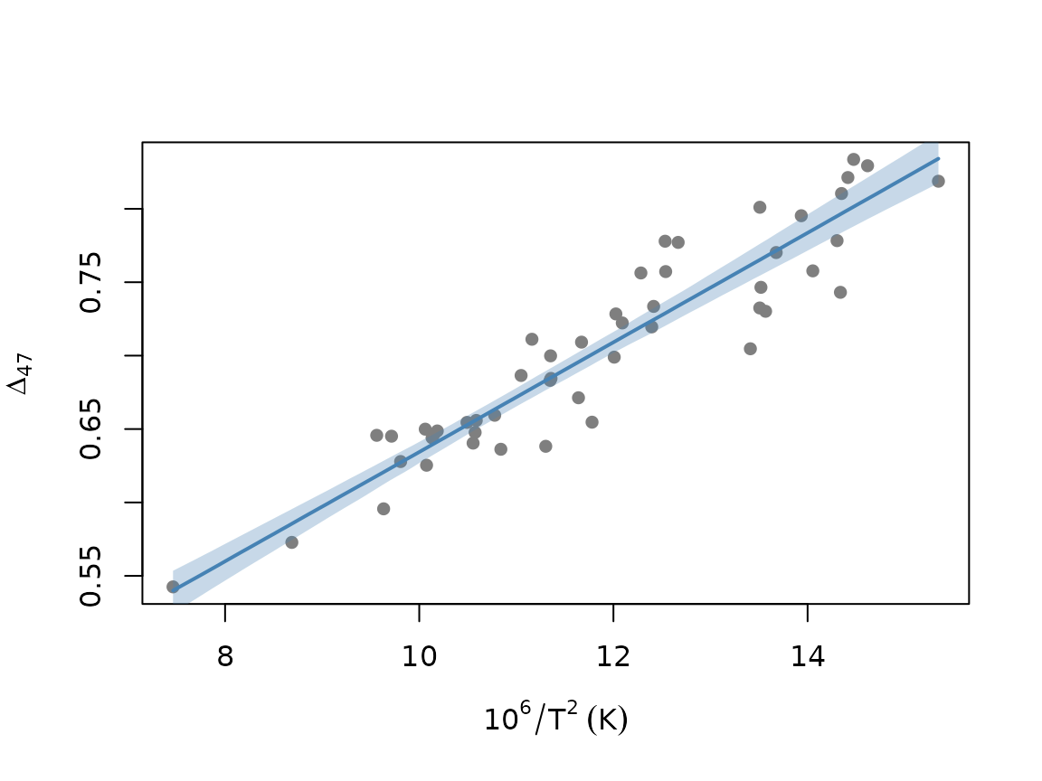
The level argument changes the probability covered by
the interval.
Reconstructing temperatures
rec.clumped() reconstructs temperatures from any of
these tables. We create a reconstruction dataset with three D47 values,
each measured with two levels of precision. Each sample has three
replicates (N):
recData <- data.frame(
  Sample = paste("Sample", 1:6),
  D47 = rep(c(0.6, 0.7, 0.8), 2),
  D47error = rep(c(0.005, 0.02), each = 3),
  N = 3
)

rec.clumped(recData = recData, obCal = fits$York)
#>     Sample D47 D47error  meanTemp        SD        SE    median      lower
#> 1 Sample 1 0.6    0.005 58.660721  4.911186  3.437023 58.689392  52.365029
#> 2 Sample 2 0.7    0.005 18.468403  3.144981  2.033767 18.499254  14.505023
#> 3 Sample 3 0.8    0.005 -9.948346  2.746298  2.140530 -9.970323 -14.304470
#> 4 Sample 4 0.6    0.020 58.660721 17.889727 10.230931 58.677627  40.359815
#> 5 Sample 5 0.7    0.020 18.468403 11.857550  6.714127 18.451745   6.318366
#> 6 Sample 6 0.8    0.020 -9.948346  8.795746  5.209176 -9.889112 -19.740435
#>       upper
#> 1 65.912565
#> 2 22.491652
#> 3 -6.006534
#> 4 80.930619
#> 5 32.399350
#> 6  0.506923
meanTemp is the temperature (°C) from the mean slope and
intercept. SE is the standard error of the temperature,
based on D47error. SD is the uncertainty of
the temperature of a single replicate, based on D47error ×
sqrt(N). median, lower, and
upper describe the 95% interval, based on
SE.
By default, both SD and SE combine the
error in D47 with the spread of slopes and intercepts in
the bootstrap. It describes the temperature predicted by the calibration
line. With prediction = TRUE, it also includes the scatter
of individual samples around that line (sigma). This is the
same kind of uncertainty given by rec.bayesian():
rec.clumped(recData = recData, obCal = fits$York, prediction = TRUE)
#>     Sample D47 D47error  meanTemp        SD        SE    median       lower
#> 1 Sample 1 0.6    0.005 58.660721 13.355650 13.100220 58.522687  36.0218934
#> 2 Sample 2 0.7    0.005 18.468403  8.920905  8.609901 18.478843   2.8886739
#> 3 Sample 3 0.8    0.005 -9.948346  6.752931  6.606941 -9.938659 -22.4203021
#> 4 Sample 4 0.6    0.020 58.660721 22.292554 16.438161 58.736171  31.7338271
#> 5 Sample 5 0.7    0.020 18.468403 14.698848 10.791817 18.531687  -0.8737733
#> 6 Sample 6 0.8    0.020 -9.948346 10.827631  8.148936 -9.919308 -24.7868063
#>       upper
#> 1 87.801710
#> 2 36.923803
#> 3  3.486241
#> 4 95.620878
#> 5 42.036172
#> 6  7.191009
We can also reconstruct the same samples under every model:
recs <- lapply(fits, function(f) rec.clumped(recData = recData, obCal = f)$meanTemp)
cbind(recData, do.call(cbind, recs))
#>     Sample D47 D47error N       OLS      WOLS    Deming      York
#> 1 Sample 1 0.6    0.005 3  59.69100  59.05976 58.719871 58.660721
#> 2 Sample 2 0.7    0.005 3  18.49426  18.45971 18.459570 18.468403
#> 3 Sample 3 0.8    0.005 3 -10.42089 -10.15967 -9.990839 -9.948346
#> 4 Sample 4 0.6    0.020 3  59.69100  59.05976 58.719871 58.660721
#> 5 Sample 5 0.7    0.020 3  18.49426  18.45971 18.459570 18.468403
#> 6 Sample 6 0.8    0.020 3 -10.42089 -10.15967 -9.990839 -9.948346